4. 2014 IOPRAO
processed with pyrnet-0.2.16
The PyrNet was setup for calibration at the DWD Lindenberg facility and the Falkenberg field from 2014-06-02 to 2014-07-18. Cross-calibration is done versus reference observations from the TROPOS MObile RaDiation ObseRvatory (MORDOR) station and BSRN measurement station at Lindeberg (Wacker & Behrens 2022).
As PyrNet stations are not clusterd on a sigle facility, but several kilometers apart, only clear sky screened reference data is used for calibration, as the sun position differences are negligible.
4.1. Imports
#|dropcode
import os
import xarray as xr
import pandas as pd
import numpy as np
import datetime as dt
import matplotlib.pyplot as plt
import jstyleson as json

from pvlib import clearsky
from pvlib.location import Location

from pyrnet import pyrnet
4.2. Prepare PyrNet data
For calibration preparation the PyrNet data is processed to level l1b using a calibration factor of 7 (uV W-1 m2) for all pyranometers with the pyrnet process l1b tool. This is done to unify the conversion to sensor voltage during calibration and not run into valid_range limits for netcdf encoding. Here we generate the calibration.json file for the processing to l1b:
box_numbers = np.arange(1,101)
calibrations = {f"{bn:03d}":[7,7] for bn in box_numbers}
calibjson = {"2000-01-01": calibrations}
with open("pyrnet_calib_prep.json","w") as txt:
    json.dump(calibjson, txt)
Within pyrnet_config.json:
{"file_calibration" : "pyrnet_calib_prep.json"}
Workflow for preparation
Prepare pyrnet_config_calibration_prep.json with contributors metadata and the dummy calibration config file.
$ pyrnet process l1a -c pyrnet_config.json raw_data/*.bin l1a/$ pyrnet process l1b_network -c pyrnet_config.json l1a/*.nc l1b_network/
4.3. Configuration
Set local data paths and lookup metadata.
pf_mordor = "mordor/{date:%Y/%m/%Y-%m-%d}_Radiation.dat"
pf_bsrn = "bsrn/{date:%Y-%m}_bsrn.tab"
pf_pyrnet = "l1b_network/{date:%Y-%m-%d}_P1D_pyrnet_ioprao_n000l1bf1s.c01.nc"
dates = pd.date_range("2014-06-04","2014-07-18")
# period with lots of clear sky situations
dates = pd.date_range("2014-06-06","2014-06-09")
stations = np.arange(1,101)

loc = Location(52.21, 14.122, altitude=125) # Lindenberg

# lookup which box contains actually a pyranometer/ extra pyranometer
mainmask = []
for box in stations:
    _, serials, _, _ = pyrnet.meta_lookup(dates[0],box=box)
    mainmask.append( True if len(serials[0])>0 else False )
4.3.1. Load reference MORDOR data
#|dropcode
#|dropout
new = True
for i,date in enumerate(dates):
    fname = pf_mordor.format(date=date)
    if not os.path.exists(fname):
        continue
    df = pd.read_csv(
        fname,
        header=0,
        skiprows=[0,2,3],
        date_format="ISO8601",
        na_values=["NAN"],
        parse_dates=[0],
        index_col=0
    )
    dst = df.to_xarray().rename({"TIMESTAMP":"time"})

    # drop not needed variables
    keep_vars = ['TP2_Wm2'] # global shortwave irradiance
    drop_vars = [v for v in dst if v not in keep_vars]
    dst = dst.drop_vars(drop_vars)
    dst = dst.resample(time="1min").mean(skipna=True)

    cs = loc.get_clearsky(pd.to_datetime(dst.time.values),model='simplified_solis')
    try:
        cs_mask = clearsky.detect_clearsky(
            dst['TP2_Wm2'].values,
            cs['ghi'],
            times=pd.to_datetime(dst.time.values)
        )
    except:
        cs_mask = np.zeros(dst.time.size).astype(bool)

    dst = dst.assign({"cs_mask":("time", cs_mask)})

    # merge
    if new:
        ds = dst.copy()
        new = False
    else:
        ds = xr.concat((ds,dst),dim='time', data_vars='minimal', coords='minimal', compat='override')

mordor = ds.copy()
mordor = mordor.drop_duplicates("time", keep="last")
mordor
<xarray.Dataset>
Dimensions:  (time: 5719)
Coordinates:
time (time) datetime64[ns] 2014-06-06 … 2014-06-09T23:18:00 Data variables: TP2_Wm2 (time) float64 0.0 0.0 0.0 0.0 0.0 0.0 … nan nan nan nan nan 0.0 cs_mask (time) bool False False False False … False False False False
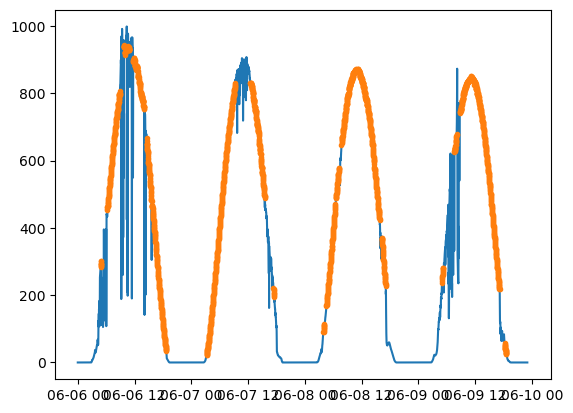
fig,ax = plt.subplots(1,1)
ax.plot(mordor.time,mordor.TP2_Wm2)
ax.plot(mordor.time[mordor.cs_mask],mordor.TP2_Wm2[mordor.cs_mask],ls='',marker='.')
[<matplotlib.lines.Line2D at 0x7efd5e626050>]
4.3.2. Load BSRN data
umonth = np.unique(dates.values.astype("datetime64[M]"))

new = True
for month in umonth:
    fname = pf_bsrn.format(date=pd.to_datetime(month))
    if not os.path.exists(fname):
        continue
    df = pd.read_csv(
        fname,
        sep='\s+',
        header=None,
        skiprows=34,
        date_format="ISO8601",
        parse_dates=[0],
        index_col=0,
        names=["time","SWD"],
        usecols=[0,2]
    )
    dst = df.to_xarray()

    dst.SWD.values[dst.SWD.values<0] = 0
    dst.SWD.values = dst.SWD.values.astype(float)

    cs = loc.get_clearsky(pd.to_datetime(dst.time.values),model='simplified_solis')

    try:
        cs_mask = clearsky.detect_clearsky(
            dst['SWD'].values,
            cs['ghi'].values,
            times=pd.to_datetime(dst.time.values),
            window_length=60
        )
    except:
        cs_mask = np.zeros(dst.time.size).astype(bool)

    dst = dst.assign({"cs_mask":("time", cs_mask)})

    # merge
    if new:
        ds = dst.copy()
        new = False
    else:
        ds = xr.concat((ds,dst),dim='time', data_vars='minimal', coords='minimal', compat='override')


bsrn = ds.copy()
bsrn = bsrn.drop_duplicates("time", keep="last")
bsrn
<xarray.Dataset>
Dimensions:  (time: 43200)
Coordinates:
time (time) datetime64[ns] 2014-06-01 … 2014-06-30T23:59:00 Data variables: SWD (time) float64 1.0 0.0 0.0 0.0 0.0 0.0 … 0.0 0.0 0.0 0.0 0.0 0.0 cs_mask (time) bool False False False False … False False False False
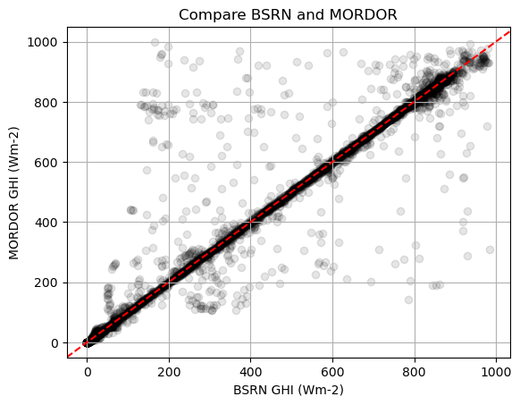
bsrnr = bsrn.interp_like(mordor)

fig,ax = plt.subplots(1,1)
ax.set_title("Compare BSRN and MORDOR")
ax.scatter(bsrnr.SWD.values, mordor.TP2_Wm2.values, alpha=0.1 ,color='k')
ax.axline((0,0),slope=1,c='r',ls='--')
ax.set_ylabel("MORDOR GHI (Wm-2)")
ax.set_xlabel("BSRN GHI (Wm-2)")

ax.grid(True)
4.3.3. Load PyrNet Data
#|dropcode
#|dropout
for i,date in enumerate(dates):
    # read from thredds server
    dst = xr.open_dataset(pf_pyrnet.format(date=date))

    # drop not needed variables
    keep_vars = ['ghi','szen']
    drop_vars = [v for v in dst if v not in keep_vars]
    dst = dst.drop_vars(drop_vars)

    # unify time and station dimension to speed up merging
    date = dst.time.values[0].astype("datetime64[D]")
    timeidx = pd.date_range(date, date + np.timedelta64(1, 'D'), freq='1s', inclusive='left')
    dst = dst.interp(time=timeidx)
    dst = dst.reindex({"station": stations})

    dst.ghi.values = dst.ghi.values * 7 * 1e-6
    dst = dst.where(dst.szen<80, drop=True)
    dst.ghi.values = dst.ghi.where(dst.ghi>0.033/300.).values

    dst = dst.resample(time="1min").mean(skipna=True)

    # merge
    if i == 0:
        ds = dst.copy()
    else:
        ds = xr.concat((ds,dst),dim='time', data_vars='minimal', coords='minimal', compat='override')

pyr = ds.copy()
pyr
<xarray.Dataset>
Dimensions:          (time: 3319, station: 43, maintenancetime: 1)
Coordinates:
station (station) int64 1 5 6 8 15 16 20 … 90 91 92 93 95 98 99
maintenancetime (maintenancetime) datetime64[ns] 2014-06-11T23:59:59
time (time) datetime64[ns] 2014-06-06T04:08:00 … 2014-06-09… Data variables: ghi (time, station) float64 0.0003242 0.0003215 … nan nan szen (time, station) float64 79.99 79.99 79.99 … 79.99 nan nan Attributes: (12/31) Conventions: CF-1.10, ACDD-1.3 title: TROPOS pyranometer network (PyrNet) observatio… history: 2024-11-12T10:03:39: Merged level l1b by pyrne… institution: Leibniz Institute for Tropospheric Research (T… source: TROPOS pyranometer network (PyrNet) references: https://doi.org/10.5194/amt-9-1153-2016 … … geospatial_lon_units: degE time_coverage_start: 2014-06-06T00:00:00 time_coverage_end: 2014-06-06T23:59:59 time_coverage_duration: P0DT23H59M59S time_coverage_resolution: P0DT0H0M1S site: [‘’, ‘’, ‘’, ‘’, ‘’, ‘’, ‘’, ‘’, ‘’, ‘’, ‘’, ‘…
4.4. Calibration
The calibration follows the ISO 9847:1992 - Solar energy — Calibration of field pyranometers by comparison to a reference pyranometer.
TODO: Revise versus 2023 EU version.
Cloudy sky treatment is applied.
4.4.1. Step 1
Drop Night measures and low signal measures from pyranometer data. Since calibration without incoming radiation doesnt work.
This data is kept for calibration:
solar zenith angle < 80° ( as recommended in ISO 9847)
Measured Voltage > 0.033 V, e.g. ADC count is 0 or 1 of 1023 (drop the lowest ~1%)
Voltage measured ($V_m$) at the logger is the amplified Senor voltage ($V_S$) by a gain of 300.
$ V_m = 300 V_S$
As the uncalibrated flux measurements ($F_U$) are calibrated with a fixed factor of 7 uV W-1 m2:
$ V_s = 71e-6 F_U $
# # Set flux values to nan if no pyranometer is installed.
# pyr.ghi.values = pyr.ghi.where(mainmask).values
4.4.2. Step 2
Interpolate reference to PyrNet samples and combine to a single Dataset
# interpolate reference to PyrNet
mordor = mordor.interp(time=pyr.time).interpolate_na()
bsrn = bsrn.interp(time=pyr.time).interpolate_na()
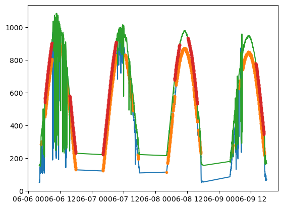
fig,ax = plt.subplots(1,1)
ax.plot(mordor.time,mordor.TP2_Wm2)
ax.plot(mordor.time[mordor.cs_mask],mordor.TP2_Wm2[mordor.cs_mask],ls='',marker='.')
ax.plot(bsrn.time,bsrn.SWD+100)
ax.plot(bsrn.time[bsrn.cs_mask],bsrn.SWD[bsrn.cs_mask]+100,ls='',marker='.')
[<matplotlib.lines.Line2D at 0x7efd5e63b190>]
# Calibration datasets for main and extra pyranometer
Cds_main = xr.Dataset(
    data_vars={
        'reference2_Wm2': ('time', mordor['TP2_Wm2'].data[bsrn.cs_mask]),
        'reference_Wm2': ('time', bsrn['SWD'].data[bsrn.cs_mask]),
        'pyrnet_V': (('time','station'), pyr['ghi'].data[bsrn.cs_mask])
    },
    coords= {
        "time": pyr.time[bsrn.cs_mask],
        "station": pyr.station
    }
)
4.4.3. Step 3
Remove outliers from series using xarray grouping and apply function. The following functions removes outliers (deviation more than 2% according to ISO 9847) from a selected group. This step involves calculating calibration series and the integration of one hour intervals to smooth out high variable situation, which would break the calibration even when time synchronization is slightly off. Also this gets rid of some random shading events like birds / chimney / rods in line of sigth, which would affect calibration otherwise. We following ISO 9847 5.4.1.1 equation (2) here.
def remove_outliers(x):
    """
    x is an xarray dataset containing these variables:
    coords: 'time' - datetime64
    'pyrnet_V' - array - voltage measures of pyranometer
    'reference_Wm2' - array - measured irradiance of reference
    """

    # calculate calibration series for single samples
    C = x['pyrnet_V'] / x['reference_Wm2']
    # integrated series
    ix = x.integrate('time')
    M = ix['pyrnet_V'] / ix['reference_Wm2']

    while np.any(np.abs(C-M) > 0.02*M):
        #calculate as long there are outliers deviating more than 2 percent
        x = x.where(np.abs(C-M) < 0.02*M)
        C = x['pyrnet_V'] / x['reference_Wm2']
        #integrated series
        ix = x.integrate('time')
        M = ix['pyrnet_V'] / ix['reference_Wm2']

    #return the reduced dataset x
    return x

# remove outliers
Cds_main = Cds_main.groupby('time.hour').apply(remove_outliers)

# hourly mean
Cds_main = Cds_main.resample(time="1h").mean(skipna=True)
4.4.4. Step 4
The series of measured voltage and irradiance is now without outliers. So we use equation 1 again to calculate from this reduced series the calibration factor for the instant samples.
C_main = 1e6*Cds_main['pyrnet_V'] / Cds_main['reference_Wm2']
C_main2 = 1e6*Cds_main['pyrnet_V'] / Cds_main['reference2_Wm2']
C_main.values[C_main.values<6]=np.nan
C_main.values[C_main.values>8]=np.nan
C_main2.values[C_main2.values<6]=np.nan
C_main2.values[C_main2.values>8]=np.nan
4.4.5. Step 5
We just found the Calibration factor to be the mean of the reduced calibration factor series and the uncertainty to be the standard deviation of this reduced series. Steo 3, 4 and 5 are done for every pyranometer seperate.
C_main_mean = C_main.mean(dim='time',skipna=True)
C_main_std = C_main.std(dim='time',skipna=True)

C_main2_mean = C_main2.mean(dim='time',skipna=True)
C_main2_std = C_main2.std(dim='time',skipna=True)
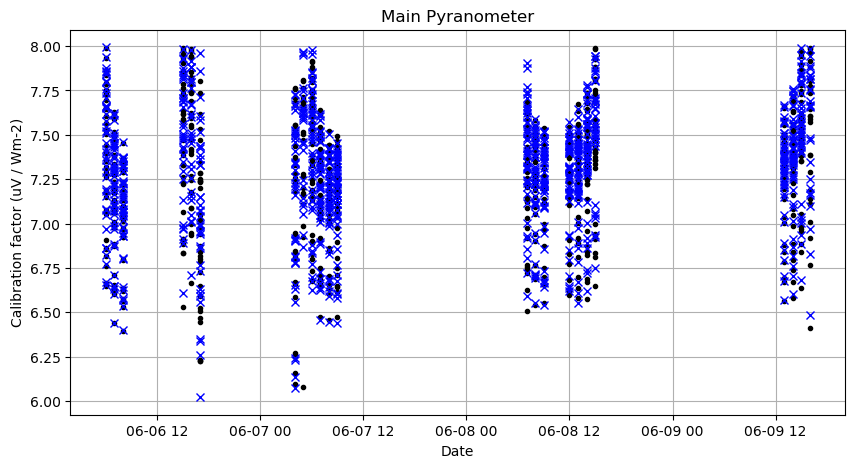
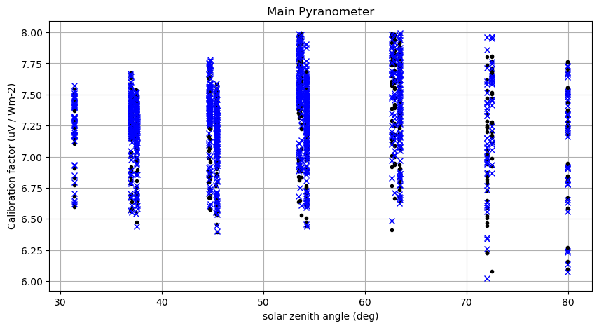
4.5. Results
#|dropcode
fig, ax = plt.subplots(1,1, figsize=(10,5))
ax.set_title("Main Pyranometer")
ax.plot(C_main.time, C_main, ls ="", marker='.',c='k')
ax.plot(C_main2.time, C_main2, ls ="", marker='x',c='b')
ax.set_xlabel("Date")
ax.set_ylabel("Calibration factor (uV / Wm-2)")
ax.grid(True)
fig.show()

plt.figure()
fig, ax = plt.subplots(1,1, figsize=(10,5))
ax.set_title("Main Pyranometer")
ax.plot(pyr.szen.interp_like(C_main), C_main, ls ="", marker='.',c='k')
ax.plot(pyr.szen.interp_like(C_main2), C_main2, ls ="", marker='x',c='b')
ax.set_xlabel("solar zenith angle (deg)")
ax.set_ylabel("Calibration factor (uV / Wm-2)")
ax.grid(True)
fig.show()
<Figure size 640x480 with 0 Axes>
calibration_new = {}
calibration2_new = {}
print(f"Box:    vs BSRN       ,      vs MORDOR ")
for box in C_main_mean.station:
    Cm = float(C_main_mean.sel(station=box).values)
    Um = float(C_main_std.sel(station=box).values)
    Cm2 = float(C_main2_mean.sel(station=box).values)
    Um2 = float(C_main2_std.sel(station=box).values)
    calibration_new.update({
        f"{box:03d}": [np.round(Cm,2), None]
    })
    calibration2_new.update({
        f"{box:03d}": [np.round(Cm2,2), None]
    })
    print(f"{box:3d}: {Cm:.2f} +- {Um:.3f} , {Cm2:.2f} +- {Um2:.3f}")

calibjson = {"2014-06-01": calibration_new}
with open("pyrnet_calib_new_bsrn.json","w") as txt:
    json.dump(calibjson, txt)

calibjson = {"2014-06-01": calibration2_new}
with open("pyrnet_calib_new_mordor.json","w") as txt:
    json.dump(calibjson, txt)
Box:    vs BSRN       ,      vs MORDOR
  1: 7.44 +- 0.198 , 7.45 +- 0.201
  5: 7.39 +- 0.300 , 7.35 +- 0.266
  6: 6.71 +- 0.253 , 6.73 +- 0.269
  8: 7.57 +- 0.346 , 7.51 +- 0.318
 15: 7.44 +- 0.217 , 7.47 +- 0.216
 16: 7.63 +- 0.190 , 7.61 +- 0.183
 20: 7.56 +- 0.196 , 7.55 +- 0.200
 21: 7.34 +- 0.224 , 7.39 +- 0.268
 22: 7.40 +- 0.219 , 7.42 +- 0.234
 30: 7.54 +- 0.230 , 7.47 +- 0.160
 37: 7.53 +- 0.174 , 7.54 +- 0.180
 41: 7.61 +- 0.206 , 7.57 +- 0.180
 42: 7.42 +- 0.280 , 7.45 +- 0.282
 43: 7.28 +- 0.161 , 7.33 +- 0.218
 44: 7.20 +- 0.399 , 7.18 +- 0.400
 45: 7.44 +- 0.243 , 7.45 +- 0.248
 46: 7.52 +- 0.261 , 7.53 +- 0.254
 47: 7.41 +- 0.254 , 7.37 +- 0.217
 49: 7.51 +- 0.225 , 7.46 +- 0.196
 50: 7.58 +- 0.199 , 7.59 +- 0.195
 53: 7.40 +- 0.301 , 7.42 +- 0.312
 54: 7.36 +- 0.305 , 7.39 +- 0.323
 55: 7.16 +- 0.237 , 7.18 +- 0.242
 56: 6.75 +- 0.188 , 6.77 +- 0.205
 57: 6.71 +- 0.198 , 6.73 +- 0.202
 61: 7.31 +- 0.205 , 7.33 +- 0.224
 64: 7.22 +- 0.178 , 7.24 +- 0.202
 68: 6.80 +- 0.142 , 6.82 +- 0.155
 71: 7.18 +- 0.228 , 7.21 +- 0.234
 74: 7.38 +- 0.080 , 7.40 +- 0.098
 75: 6.64 +- 0.158 , 6.63 +- 0.208
 80: 6.90 +- 0.176 , 6.92 +- 0.187
 82: 7.42 +- 0.187 , 7.43 +- 0.175
 86: 7.37 +- 0.157 , 7.40 +- 0.186
 87: 7.32 +- 0.205 , 7.34 +- 0.224
 88: 6.90 +- 0.205 , 6.92 +- 0.183
 90: 7.36 +- 0.218 , 7.38 +- 0.204
 91: 7.40 +- 0.244 , 7.45 +- 0.273
 92: 7.08 +- 0.280 , 7.16 +- 0.196
 93: 7.50 +- 0.161 , 7.52 +- 0.189
 95: 7.44 +- 0.253 , 7.46 +- 0.278
 98: 7.13 +- 0.240 , 7.15 +- 0.248
 99: 7.38 +- 0.193 , 7.40 +- 0.207