3. 2015 MelCol
processed with pyrnet-0.2.16
The PyrNet was setup for calibration in a dense array on the Melpitz measurement field from 2015-05-06 to 2015-05-11. Cross-calibration is done versus reference observations from the TROPOS MObile RaDiation ObseRvatory (MORDOR) station.
3.1. Imports
#|dropcode
from IPython.display import display, Latex
import os
import xarray as xr
import pandas as pd
import numpy as np
import datetime as dt
import matplotlib.pyplot as plt
import jstyleson as json

from scipy.optimize import differential_evolution

from pvlib import clearsky
from pvlib.location import Location

import pyrnet.pyrnet
import pyrnet.utils
3.2. Prepare PyrNet data
For calibration preparation the PyrNet data is processed to level l1b using a calibration factor of 7 (uV W-1 m2) for all pyranometers with the pyrnet process l1b tool. This is done to unify the conversion to sensor voltage during calibration and not run into valid_range limits for netcdf encoding.
Before running this notebook, new absolute calibration factors have to be determined with calibration_melcol.ipynb
3.3. Configuration
Set local data paths and lookup metadata.
pf_mordor = "mordor/{date:%Y-%m-%d}_Radiation.dat"
pf_pyrnet = "l1b_network/{date:%Y-%m-%d}_P1D_pyrnet_melcol_n000l1bf1s.c01.nc"
dates = pd.date_range("2015-05-06","2015-05-11")

loc = Location(51.525175, 12.91648, altitude=90) # Melpitz

stations = np.arange(1,101)
# lookup which box contains actually a pyranometer/ extra pyranometer
mainmask = []
for box in stations:
    _, serials, _, _ = pyrnet.pyrnet.meta_lookup(dates[0],box=box)
    mainmask.append( True if len(serials[0])>0 else False )
3.3.1. Load reference MORDOR data
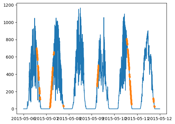
The reference data of MORDOR is loaded, and clearsky is detected on daily basis using solis_simple clearsky model and the pvlib.clearsky.detect_clearsky function.
#|dropcode
#|dropout
for i,date in enumerate(dates):
    fname = pf_mordor.format(date=date)
    df = pd.read_csv(
        fname,
        header=0,
        skiprows=[0,2,3],
        date_format="ISO8601",
        parse_dates=[0],
        index_col=0
    )
    dst = df.to_xarray().rename({"TIMESTAMP":"time"})

    # drop not needed variables
    keep_vars = ['TP2_Wm2'] # GHI,DHI,DNI
    drop_vars = [v for v in dst if v not in keep_vars]
    dst = dst.drop_vars(drop_vars)
    dst = dst.drop_duplicates("time",keep="last")
    dst = dst.resample(time="1min").mean(skipna=True)

    cs = loc.get_clearsky(pd.to_datetime(dst.time.values),model='simplified_solis')
    try:
        cs_mask = clearsky.detect_clearsky(
            dst['TP2_Wm2'].values,
            cs['ghi'],
            times=pd.to_datetime(dst.time.values)
        )
    except:
        cs_mask = np.zeros(dst.time.size).astype(bool)

    dst = dst.assign({"cs_mask":("time", cs_mask)})
    # merge
    if i == 0:
        ds = dst.copy()
    else:
        ds = xr.concat((ds,dst),dim='time', data_vars='minimal', coords='minimal', compat='override')

mordor = ds.copy()
mordor = mordor.drop_duplicates("time", keep="last")
mordor
<xarray.Dataset>
Dimensions:  (time: 8640)
Coordinates:
time (time) datetime64[ns] 2015-05-06 … 2015-05-11T23:59:00 Data variables: TP2_Wm2 (time) float64 0.0 0.0 0.0 0.0 0.0 0.0 … 0.0 0.0 0.0 0.0 0.0 0.0 cs_mask (time) bool False False False False … False False False False
plt.plot(mordor.time,mordor.TP2_Wm2)
plt.plot(mordor.time[mordor.cs_mask],mordor.TP2_Wm2[mordor.cs_mask],ls='',marker='.')
[<matplotlib.lines.Line2D at 0x7ff685cadc90>]
3.3.2. Load PyrNet Data
#|dropcode
#|dropout
for i,date in enumerate(dates):
    # read from thredds server
    dst = xr.open_dataset(pf_pyrnet.format(date=date))
    # drop not needed variables
    keep_vars = ['ghi','szen']
    drop_vars = [v for v in dst if v not in keep_vars]
    dst = dst.drop_vars(drop_vars)

    # unify time and station dimension to speed up merging
    date = dst.time.values[0].astype("datetime64[D]")
    timeidx = pd.date_range(date, date + np.timedelta64(1, 'D'), freq='1s', inclusive='left')
    dst = dst.interp(time=timeidx)
    dst = dst.reindex({"station": stations})

    # merge
    if i == 0:
        ds = dst.copy()
    else:
        ds = xr.concat((ds,dst),dim='time', data_vars='minimal', coords='minimal', compat='override')

pyr = ds.copy()
pyr
<xarray.Dataset>
Dimensions:          (station: 100, maintenancetime: 50, time: 518400)
Coordinates:
station (station) int64 1 2 3 4 5 6 7 8 … 94 95 96 97 98 99 100
maintenancetime (maintenancetime) datetime64[ns] 2015-05-12T07:55:50 ……
time (time) datetime64[ns] 2015-05-06 … 2015-05-11T23:59:59 Data variables: ghi (time, station) float64 0.0 nan nan 0.0 … nan 0.0 0.0 nan szen (time, station) float64 111.0 nan nan … 109.4 109.4 nan Attributes: (12/31) Conventions: CF-1.10, ACDD-1.3 title: TROPOS pyranometer network (PyrNet) observatio… history: 2024-11-04T23:59:36: Merged level l1b by pyrne… institution: Leibniz Institute for Tropospheric Research (T… source: TROPOS pyranometer network (PyrNet) references: https://doi.org/10.5194/amt-9-1153-2016 … … geospatial_lon_units: degE time_coverage_start: 2015-05-06T00:00:00 time_coverage_end: 2015-05-06T23:59:59 time_coverage_duration: P0DT23H59M59S time_coverage_resolution: P0DT0H0M1S site: [‘’, ‘’, ‘’, ‘’, ‘’, ‘’, ‘’, ‘’, ‘’, ‘’, ‘’, ‘…
3.4. Calibration
The calibration follows the ISO 9847:1992 - Solar energy — Calibration of field pyranometers by comparison to a reference pyranometer. For selecting and masking the data.
TODO: Revise versus 2023 EU version.
Cloudy sky treatment is applied.
3.4.1. Step 1
Drop Night measures and low signal measures from pyranometer data. Since calibration without incoming radiation doesnt work.
This data is kept for calibration:
solar zenith angle < 80° ( as recommended in ISO 9847)
Measured Voltage > 0.033 V, e.g. ADC count is 0 or 1 of 1023 (drop the lowest ~1%)
Voltage measured ($V_m$) at the logger is the amplified Senor voltage ($V_S$) by a gain of 300.
$ V_m = 300 V_S$
As the uncalibrated flux measurements ($F_U$) are calibrated with a fixed factor of 7 uV W-1 m2:
$ V_s = 71e-6 F_U $
# Set flux values to nan if no pyranometer is installed.
pyr.ghi.values = pyr.ghi.where(mainmask).values

# convert to measured voltage
pyr.ghi.values = pyr.ghi.values * 7 * 1e-6

# Step 1, select data
pyr = pyr.where(pyr.szen<80, drop=True)
pyr.ghi.values = pyr.ghi.where(pyr.ghi>0.033/300.).values
3.4.2. Step 2
Apply new absolute calibration from calibration_melcol.ipynb
calib_new = pyrnet.utils.read_json("pyrnet_calib_new.json")
calib_new = calib_new[list(calib_new.keys())[0]]
for station in pyr.station:
    pyr.ghi.sel(station=station).values /= calib_new[f"{station:03d}"][0] * 1e-6
3.4.3. Step 3
Interpolate reference to PyrNet samples and combine to a single Dataset
# interpolate reference to PyrNet
mordor = mordor.interp(time=pyr.time).interpolate_na()


# Calibration datasets for main and extra pyranometer
Cds_main = xr.Dataset(
    data_vars={
        'reference_Wm2': ('time', mordor['TP2_Wm2'].data[mordor.cs_mask]),
        'pyrnet_Wm2': (('time','station'), pyr['ghi'].data[mordor.cs_mask,:]),
        'szen': ('time',pyr.szen.mean("station",skipna=True).data[mordor.cs_mask])
    },
    coords= {
        "time": pyr.time[mordor.cs_mask],
        "station": pyr.station
    }
)
3.4.4. Step 4
Remove outliers from series using xarray grouping and apply function.
def remove_outliers(x):
    """
    x is an xarray dataset containing these variables:
    coords: 'time' - datetime64
    'pyrnet_V' - array - voltage measures of pyranometer
    'reference_Wm2' - array - measured irradiance of reference
    """

    # calculate calibration series for single samples
    C = x['pyrnet_Wm2'] / x['reference_Wm2']
    # integrated series
    ix = x.integrate('time')
    M = ix['pyrnet_Wm2'] / ix['reference_Wm2']

    while np.any(np.abs(C-M) > 0.01*M):
        #calculate as long there are outliers deviating more than 2 percent
        x = x.where(np.abs(C-M) < 0.01*M)
        C = x['pyrnet_Wm2'] / x['reference_Wm2']
        #integrated series
        ix = x.integrate('time')
        M = ix['pyrnet_Wm2'] / ix['reference_Wm2']

    #return the reduced dataset x
    return x

# remove outliers
Cds_main = Cds_main.groupby('time.hour').apply(remove_outliers)

# hourly mean
Cds_main = Cds_main.coarsen(time=60*60,boundary='trim').mean(skipna=True)
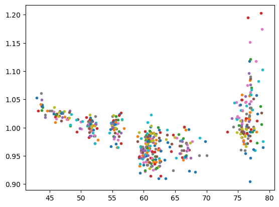
3.4.5. Step 5
The series of measured reference and pyrnet irradiance is now without outliers. Now we can fit a cubic function - (reference/pyrnet) vs. szen - to determine the cosine correction function for pyrnet.
fig,ax = plt.subplots(1,1)
p = ax.plot(Cds_main.szen,Cds_main.reference_Wm2/Cds_main.pyrnet_Wm2,ls='',marker='.')
def cubic_function(x, a, b, c, d):
    return a * x ** 3 + b * x ** 2 + c * x + d

def objective_function(coefficients, x, y):
    a, b, c, d = coefficients
    y_pred = cubic_function(x, a, b, c, d)
    error = np.sum((y - y_pred) ** 2)
    return error
bounds = [(-5, 5), (-5, 5), (-5, 5), (-5, 5)]


ratio = Cds_main.reference_Wm2/Cds_main.pyrnet_Wm2

result = differential_evolution(
    objective_function,
    args=(np.cos(np.deg2rad(Cds_main.szen)), ratio),
    bounds=bounds,
    seed=1
)
result
 message: Optimization terminated successfully.
 success: True
     fun: 0.39807904993609633
       x: [-2.335e+00  4.402e+00 -2.437e+00  1.379e+00]
     nit: 56
    nfev: 3545
     jac: [ 2.380e-04  4.970e-04  7.820e-04  1.921e-04]
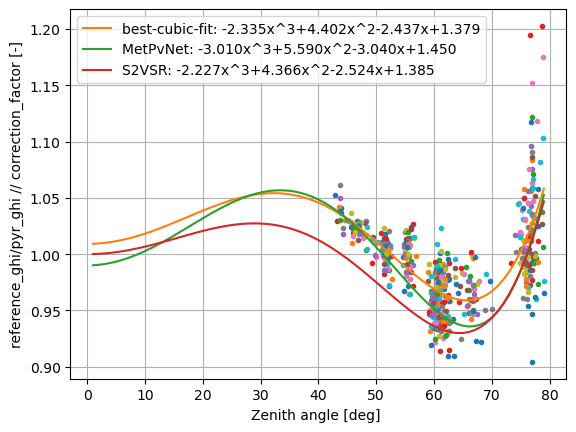
3.5. Results
print("Best cubic fit:")
a3, a2, a1, a0 = result.x
display(Latex(
    rf"""
    {a3:+.3f}x^3{a2:+.3f}x^2{a1:+.3f}x{a0:+.3f}
    """
))
Best cubic fit:


-2.335x^3+4.402x^2-2.437x+1.379
# Coefficients from other calibrations:

display(Latex(
    rf"""
    MelCol: {a3:+.3f}x^3{a2:+.3f}x^2{a1:+.3f}x{a0:+.3f}
    """
))

b3, b2, b1, b0 = [ -3.01, 5.59, -3.04, 1.45 ]
display(Latex(
    rf"""
    MetPVNet: {b3:+.3f}x^3{b2:+.3f}x^2{b1:+.3f}x{b0:+.3f}
    """
))
c3, c2, c1, c0 = [ -2.227, 4.366, -2.524, 1.385 ]
display(Latex(
    rf"""
    S2VSR: {c3:+.3f}x^3{c2:+.3f}x^2{c1:+.3f}x{c0:+.3f}
    """
))
MelCol: -2.335x^3+4.402x^2-2.437x+1.379


MetPVNet: -3.010x^3+5.590x^2-3.040x+1.450


S2VSR: -2.227x^3+4.366x^2-2.524x+1.385
szen = np.arange(1,80)
mu0 = np.cos(np.deg2rad(szen))

fig,ax = plt.subplots(1,1)
p = ax.plot(Cds_main.szen,Cds_main.reference_Wm2/Cds_main.pyrnet_Wm2,ls='',marker='.')
ax.plot(szen, a3*mu0**3 + a2*mu0**2 + a1*mu0 + a0,
         color='C1', label=f'best-cubic-fit: {a3:+.3f}x^3{a2:+.3f}x^2{a1:+.3f}x{a0:+.3f}')
ax.plot(szen, b3*mu0**3 + b2*mu0**2 + b1*mu0 + b0,
         color='C2', label=f'MetPvNet: {b3:+.3f}x^3{b2:+.3f}x^2{b1:+.3f}x{b0:+.3f}')
ax.plot(szen, c3*mu0**3 + c2*mu0**2 + c1*mu0 + c0,
         color='C3', label=f'S2VSR: {c3:+.3f}x^3{c2:+.3f}x^2{c1:+.3f}x{c0:+.3f}')

ax.legend()
ax.set_xlabel('Zenith angle [deg] ')
ax.set_ylabel('reference_ghi/pyr_ghi // correction_factor [-]')
ax.grid(True)
# dump to json
calibjson = {"2015-05-06": {"CC":list(result.x[::-1])}}
with open("pyrnet_calib_cc_new.json","w") as txt:
    json.dump(calibjson, txt)